Newtons Logistic Regression

Stories, Articles, Arts, Poems, Fictions
Newtons Logistic Regression
This article provides results, graphical plots and analysis of Linear, Logistic Regression, Naive Bayes for three kinds of datasets, namely, (i) Linearly Seperable, (ii) Non-Linearly Seperable and (iii) Banana Data. This article plays a good role for new mentors, academicians and students to understand the process of experimentations and analysis, result presentation in a Machine Learning tasks. It also plots the classifier hyperplane along with the distinct class in this 2-class problem. The results are not benchmarks, they are elaborated for experimental setups in labs, and to be followed by mentors teaching Machine Learning Lab Work. For benchmark results look into peer-reviewed research papers.
Here some results obtained after the dividing the data into 30-70 ratio of testing and training respectively. This was done for 5 folds. Finally, average was taken. This has been done for all thre classifiers who’s results are discussed below.
The following table shows results for linearly seperable data for the three classifiers (i) Linear Regression (ii) Logistic Regression and (iii) Naïve Bayes. The results are averages over 5 folds and are comparable.
Following are the plots of given data.

Non Linearly Seperable Data plot


LS Data Results (Note the data are averages of 5 fold data)
| TP | TN | FP | FN | Precision | Recall | F-Value | Accuracy | |
| Linear Regression | 750 | 750 | 0 | 0 | 1 | 1 | 1 | 1 |
| Logistic regression | 749.6 | 750 | 0 | 0.4 | 1 | 0.9995 | 0.9997 | 0.9997 |
| Naïve Bayes | 750 | 750 | 0 | 0 | 1 | 1 | 1 | 1 |
The following table shows results for non linearly seperable data for the three classifiers (i) Linear Regression (ii) Logistic Regression and (iii) Naïve Bayes. The best results are with Linear and logistic regression.
NLS Data Results (Note the data are averages of 5 fold data)
| TP | TN | FP | FN | Precision | Recall | F-Value | Accuracy | |
| Linear Regression | 735.5 | 734.8000 | 15.2000 | 14.6000 | 0.9797 | 0.9805 | 0.9801 | 0.9801 |
| Logistic regression | 733.8 | 733.2000 | 16.8000 | 16.2000 | 0.9776 | 0.9784 | 0.9780 | 0.9780 |
| Naïve Bayes | 721 | 726 | 29 | 24 | 0.965 | 0.965 | 0.888 | 0.96 |
The following table shows results for banana data for the three classifiers (i) Linear Regression (ii) Logistic Regression and (iii) Naïve Bayes. The results are averages over 5 folds and Naive Bayes gives the best results.
| TP | TN | FP | FN | Precision | Recall | F-Value | Accuracy | |
| Linear Regession | 626.4000 | 633.8000 | 122.2000 | 116.6000 | 0.8370 | 0.8431 | 0.8399 | 0.8407 |
| Logistic Regression | 665 | 515 | 240 | 78 | 0.7425 | 0.8950 | 0.8094 | 0.7876 |
| Naïve Bayes | 666 | 666 | 96 | 72 | 0.88 | 0.88 | 0.888 | 0.88 |
The surfaces and figures of the discriminant are given below.
Below are the two plots of linearly separable data surface generated by linear regression. The two plots have different axis coordinates.


Below are the two plots of non linearly separable data surface generated by linear regression. The two plots have different axis coordinates.


Below are the two plots of banana data surface generated by linear regression. The two plots have different axis coordinates.


Below are the two plots of linearly separable data surface generated by logistic regression. The two plots with different runs and different training and testing data.
The following are surface generated over two runs.


Below are the two plots of non linearly separable data surface generated by logistic regression.

Below are the two plots of banana data surface generated by logistic regression. The two plots with different runs and different training and testing data.
(The outputs are over two runs)


Now the samples of training sizes (500, 1000, 1500,….,4500) and {{5000}-{training-size}} as the testing size is being analyzed here. I iterate over with incrementing each time the partition(train-test ratio) percentage by 0.1% of 5000 to .2% of 5000 and so on to -9% of 5000, remaining to be for testing. This is how we will get the training size of (500, 1000, 1500, ……,4500)and testing ratio as 5000-{training-size}.
Average time over 5 such samples of each of the given training size. Following are the experiment results of execution times. Of different algorithms and different data sets.
I have converted data to 1 and 0 class instead of 1 and -1 class before using logit. Following are the results of logistic regression of all the three data samples (i)Banana Data (ii) NLS Data and (iii) LS Data.
In the below table the training sizes are given and the corresponding testing sizes are 5000-{training size}
| Testing Sample | 4500 | 4000 | 3500 | 3000 | 2500 | 2000 | 1500 | 1000 | 500 |
| Banana Data | 3.5992 | 2.7031 | 2.8467 | 2.6833 | 1.4648 | 1.1170 | 1.0087 | 0.6808 | 0.4955 |
| NLS Data | 3.5631 | 3.3242 | 3.4129 | 3.1384 | 3.3511 | 1.5047 | 1.4308 | 0.8716 | 0.5782 |
| LS Data | 0.4260 | 0.3063 | 0.1808 | 0.6101 | 0.3813 | 0.0842 | 0.2085 | 0.0642 | 0.0364 |
Following are the results of linear regression of all the three data samples (i)Banana Data (ii) NLS Data and (iii) LS Data
| Training Sample | 4500 | 4000 | 3500 | 3000 | 2500 | 2000 | 1500 | 1000 | 500 |
| Banana Data | 0 | 0 | 0 | 0 | 0 | 0.0633 | 0 | 0 | 0 |
| NLS Data | 0 | 0.0989 | 0 | 0 | 0.1900 | 0.0570 | 0 | 0 | 0 |
| LS Data | 0 | 0 | 0 | 0 | 0 | 0.0566 | 0 | 0 | 0 |
To use Naïve Bayes I have used discretizer present in weka before applying Naïve Bayes. Following are the results of Nayes Bayes of all the three data samples (i)Banana Data (ii) NLS Data and (iii) LS Data.
| Training Sample | 4500 | 4000 | 3500 | 3000 | 2500 | 2000 | 1500 | 1000 | 500 |
| Banana Data | 0 | 0 | 0.02 | 0.02 | 0.02 | 0 | 0 | 0.02 | 0 |
| NLS Data | 0 | 0 | 0 | 0.02 | 0.02 | 0.02 | 0 | 0.02 | 0.02 |
| LS Data | 0 | 0.02 | 0 | 0 | 0.02 | 0 | 0 | 0 | 0.02 |
First Order Polynomial Fitting for NLS Data:-
I have used polyfit and polyval for this part
Each is linear in number of Samples . ie O(N).
I have computer x = x1*x1+y1*y1
And used polyfit the parameter with 1 degree polyfit are:-
-0.0237x+ 1.4974. Graph Below

With x1 I am getting the parameter with 1 degree polyfit are:-
-0.2301 x+ 1.5416. Graph below

With x2 I am getting the parameter with 1 degree polyfit are:-
I have computer x = x1*x1+y1*y1
And used polyfit the parameter with 1 degree polyfit are:-
-0.0081x+ 1.2010
With x1 I am getting the parameter with 1 degree polyfit are:-
-0.1628x+ 1.4918
With x2 I am getting the parameter with 1 degree polyfit are:-
-0.1684x+ 1.4518
x = x1*x1+y1*y1
And used polyfit the parameter with 1 degree polyfit are:-
0+-0.0151 x+1.4139
This is almost linear
With x1 I am getting the parameter with 1 degree polyfit are:-
-0.0041x^2+-0.1254x + 1.4189
This is almost linear
With x2 I am getting the parameter with 1 degree polyfit are:-
0.0003x^2 -0.17702x+ 1.5425
This is also almost straight line
So polynomial of degree 1 fits in Logistic regression and similar results were coming for linear regression
| Linear Regression | Parameters of polyfit for degree 1 with x = x1*x1+y1*y1 | Parameters of polyfit for degree 1 with x = x1 | Parameters of polyfit for degree 1 with x = x2 |
| NLS Data | -0.0237x+ 1.4974 | -0.2301x+ 1.5416 | 1.709x+2.0415 |
| LS Data | -0.0018x+ 1.2346 | -0.1477x+ 1.5013 | -0.1794x+1.9014 |
| Banana Data | -0.0129x+ 2.2202 | -0.2264x+ -1.4032 | 0.9265x+ -1.6075 |
| Logistic Regression | Parameters of polyfit for degree 1 with x = x1*x1+y1*y1 | Parameters of polyfit for degree 1 with x = x1 | Parameters of polyfit for degree 1 with x = x2 |
| NLS Data | -0.0081x+ 1.2010 | -0.1628x+ 1.4918 | -0.1684x+1.4518 |
| LS Data | -0.0020x+ 1.0548 | -0.0794x+ 1.2986 | -0.0785x+1.2847 |
| Banana Data | -0.0021x+ 0.8505 | 0.0438x+ 0.5558 | 0.0191x+ 0.5530 |
The following are results obtained using the logistic regression using Newton’s method classifier. I have split the datasets into 70% training and 30% testing randomly in 5 folds. Below are the details of how we choose these 5 folds.
Here the first weight represent the bias
sum = sum + W_Old(j+1)*trainingSet(t,j);
P(t) = 1/(1+ exp(-1*sum));
Z= (X’) * (Y-P)’;
W = diag(P.* (1-P));
Hessian = X’ * W * X;
etaMatrix(1:3) = eta;
W_New = W_Old + etaMatrix .* (Hessian \ Z)’ ;
Its derivation and complete form in two ways is given as:

Parameters used for computations:
Maximum Number of numIteration =10000;
eta = 0.5 and 0.2; // both tested
errorBound = 0.0001;
The following are the final weights for the three data:-
| W0 | W1 | W2 | |
| LS Data | 8.4137 | -0.4298 | -0.4125 |
| NLS Data | 26.2879 | -2.2458 | -2.1134 |
| Banana Data | 0.6495 | 0.3533 | -0.1829 |
The following are the TP, TN , FP, FN, Precision, recall, accuracy for the three data:
| TP | TN | FP | FN | Precision | Recall | F-Value | Accuracy | |
| LS Data | 750 | 750 | 0 | 0 | 1 | 1 | 1 | 1 |
| NLS Data | 737.6 | 732.8 | 17.2 | 12.4 | 0.9772 | 0.9835 | 0.9835 | 0.9803 |
| Banana Data | 630.6 | 647.4 | 108.6 | 112.4 | 0.8531 | 0.8487 | 0.8509 | 0.8526 |
The Decision Boundaries of the three data sets are as follows:-
The following are the figues showing (i) the decision surface and (ii) decision surface and dat both. Note different colored are used to show different classes.
This following figure is for the plane of the Newtons method for linearly seperable data. Red dots shows the predicted line projected in 2D

This following figure is for data for linearly separable data.

This following figure is for the plane of the Newtons method for linearly seperable data plotted in 3D

This following figure is for the data for non linearly seperable data.

This following figure is of the Newtons method for NLS seperable data. Red dots shows the predicted line projected in 2D.

This figure is for the plane of the Newtons method for non linearly seperable data over two runs.


This following figure is for the separating plane of the Newtons method for banana data.

This following figure is for the plane of the Newtons method for banana data projected to 2D.

This figure is for the plane of the Newtons method for banana data. Red dots shows the predicted line projected in 2D

The results are self explanatory with the help of image data and are not benchmarks, they are elaborated for experimental setups in labs, and to be followed by mentors teaching Machine Learning Lab Work. For benchmark results look into peer-reviewed research papers.
% this is for two class problem for more than two class code changes
% % this is for two class problem for more than two class code changes
% % ————-Parameters————-
% numIteration =1000; The Number of maximum iterations
% % errorBound = 0.0001; This is the permissible error.
% The experiments have been done keep in view both the error condition
% reached or maximum iteration reached whichever comes first.
% % eta = 0.5; This is the learning rate, experiments have been
% done on various learning rates
function logisticRegression2Class()
disp(‘..Starting logistic regression Algorithm….’);
%reading the data

A = load('BananaData.mat');
data = A.data;
[N,col]= size(data);

vtot=[0, 0, 0, 0,0, 0,  0 , 0];

%5 folds with 70-30 ratio
for i = 1:5
    P=.3;
    groups=data(:,3);
    [train,test] = crossvalind('holdout',groups, P);
    train1= data(train, 1: 3);
    test1=data(test, 1:3);
    [trainLengthRow, trainLengthCol]=size(train1);
    [rowtest,coltest]= size(test1);

    trainingSet = train1(1:trainLengthRow, 1 : trainLengthCol -1 );
    trainingLabels = train1(1:trainLengthRow, trainLengthCol );

    testSet = test1(1:rowtest, 1 : coltest -1 );
    testLabels = test1(1:rowtest, coltest );

%initilizating weights
weights(1:trainLengthCol) = 0;
weight0=0;
[weight0, weights] = trainLogReg(weight0, weights, trainingSet,trainingLabels);
[correctlyClassified,count0,count1,unClassified,v] = testLogReg(testSet,testLabels, weight0, weights)
vtot = vtot +v ;
end
disp(‘TP, TN, FP, FN, TP/(TP+FP), TP/P, 2PR / (P+R) , correctlyClassified/trainLengthRow’);
vtot = vtot ./ 5
end
%This mathod is for tarining the logestic regression problem
% —–Parameters—-
%trainingSet: the training set
%trainingLabels: the labels corresponding to the traiining set
%weights: the initial weights obtained from traiining
%weight0: The initial bias weight
%—–Return Types——
%weights: the final weights obtained from traiining
%weight0: The bias weight
%
function [weight0, weights] = trainLogReg(weight0, weights, trainingSet,trainingLabels)
numIteration =100000;
eta = 0.5;
errorBound = 0.0001;
error =1.0;
[trainLengthRow, trainLengthCol] = size(trainingSet);
del_l_by_del_w_i(1:trainLengthCol) = 0;
weightsFinal(1:trainLengthCol) = 0;
k=0
while ((k < numIteration) && (error > errorBound))
    error=0.0;
for i=1:trainLengthCol
    Y1_X = 0;
    del_l_by_del_w_i(i) = 0;
    del_l_by_del_w_0 = 0;

    for t=1: trainLengthRow
        sum = weight0;

        for j=1: trainLengthCol
        sum = sum +  weights(j)*trainingSet(t,j);
        end;

        Y1_X = 1/(1+ exp(-1*sum));

        del_l_by_del_w_i(i) = del_l_by_del_w_i(i) + trainingSet(t,i) *(trainingLabels(t) - Y1_X ) ;
        del_l_by_del_w_0 = del_l_by_del_w_0 + 1 *(trainingLabels(t) - Y1_X ) ;
    end;

end;

for i=1:trainLengthCol
weightsFinal(i)= weights(i) + eta *  del_l_by_del_w_i(i);
error = error + (weightsFinal(i)-weights(i))*(weightsFinal(i)-weights(i));
end;

weight0new = weight0 +    eta *  del_l_by_del_w_0;
error = error + (weight0new-weight0)*(weight0new-weight0);
error=sqrt(error);
weights=weightsFinal;
weight0 = weight0new;
k=k+1;
end

k
%Now computing the final y using the final weights

y1(1:trainLengthRow)=0;
y0(1:trainLengthRow)=0;

for i =1: trainLengthRow

    sum = weight0;

    for j=1: trainLengthCol
    sum = sum +  weightsFinal(j)*trainingSet(i,j);
    end;

    y1(i) = 1/(1+ exp(-1*sum));
    y0(i) = 1/(1+ exp(sum));

 end;
% Following is the code for plotting the data
% data(1:trainLengthRow, 1:trainLengthCol+1)=0;
% data(1:trainLengthRow, 1:trainLengthCol)= trainingSet;
% for p=1:trainLengthRow
% data(p, trainLengthCol+1)= y1(p);
% end;
%
% %figure
% % parallelcoords(data,’Labels’,labels);
%
% for p=1:trainLengthRow
% x1(p)= trainingSet(p,1);
% end;
%
% for p=1:trainLengthRow
% x2(p)= trainingSet(p,2);
% end;
%
%
% for p=1:trainLengthRow
% yOrginal(p)= trainingLabels(p);
% end;
%
%
% size(x1)
% size(x2)
% size(trainingLabels)
%
% figure
% scatter3(x1,x2,trainingLabels,10);
% axis([-10,10,-10,10,-10,10])
%
% figure
% plot3(x1,x2,y1);
% axis([-10,10,-10,10,-10,10])
%
%
% xx=[-10:1:10];
% yy=[-10:1:10];
% [xx1,yy1]=meshgrid(xx,yy);
%
% sum = -1 .* (weight0+weightsFinal(1).xx1+weightsFinal(2).yy1);
% zz= 1 ./(1 + expm(sum));
% figure
% surf(xx1,yy1,zz);
% title(‘title’);
% xlabel(‘x’);
% ylabel(‘y’)
% zlabel(‘z’);
end
%This is the method that is called to test the accuracy of the methods
%———————–Parameters————————–
%testSet: the set of samples to be considered for testing
%testLabels: the labels corresponding to testset
%weight0, weight: the weights corresponding to logistic regression
%———————–Return Values————————
%correctlyClassified: The number of correctly classified samples
%unClassified: The array containing 5 unclassified data samples from each
%classification type
%v: The vecor that returns the computed values of TP;TN; FP; FN ,P; R; F, accuracy
function [correctlyClassified,count0,count1,unClassified,v] = testLogReg(testSet,testLabels, weight0, weights)
correctlyClassified = 0;
count0 = 0; count1=0;   TP=0;    TN=0;     FP=0;     FN =0; P=0; R=0; F=0;

[testLengthRow,testLengthCol]=size(testSet);
unClassified(1:10 ,1: testLengthCol) = 0;

% checking accuracy by  number of correctly classified

for k=(1: testLengthRow )
    x=[1, testSet(k,1:testLengthCol)];
    w =[weight0,weights];
    O1=    x' .* w' ;

    %computing the value of vector with plane
    sum =0;
    for p=1:length(O1)
        sum = sum +O1(p);
    end

     y1x = 1/(1+ exp(-1*sum));
     if(y1x>=0.5)
         %disp('class 1');
         O =1;
     else
         %disp('class 0');
         O =-1;
     end

     %    error as output approaching target
    if (O == testLabels(k))
        % correctly classified examples
        correctlyClassified=correctlyClassified+1;

        %compute  TP, TN
        if(testLabels(k)==1)
            TP = TP+1;
        else
            TN = TN +1;
        end

    else
        % wrongly classified examples
        if(testLabels(k)==1)
            FN = FN+1;
        else
            FP = FP +1;
        end
        %storing 5 misclassified  classes from each class
        if(count1<5 && testLabels(k)==1)
            count1 = count1 + 1;
            unClassified(count1,1: testLengthCol) = testSet(k,1: testLengthCol);
        end
        if(count0<5 && testLabels(k)==-1 )
            count0 = count0 + 1;
            unClassified(count0,1: testLengthCol) = testSet(k,1: testLengthCol);
        end
    end

end

  k
P= TP/(TP+FP)
R=  TP/(TP+FN)
v=[TP,    TN,     FP,     FN,     P,     R,      2*P*R / (P+R) , correctlyClassified/testLengthRow]
disp('TP,    TN,     FP,     FN,     TP/(TP+FP),      TP/P,      2*P*R / (P+R) , correctlyClassified/trainLengthRow');


 unClassified;
 accuracy = correctlyClassified/testLengthRow  ;
 accuracy
end
Preprocessing: I have created three .mat files from the given input in form of a text file. I first imported it in xls and then copied it to .mat files.
NOTE: The derivation for linear and logistic regression is added at the end of the document.
I have split the datasets into 70% training and 30% testing randomly in 5 folds. I have used matlab method crossvalind to create 70-30 ratio of training and testing and did this 5 times. Finally I calculated the average over the five runs.
Now the details of form I have used for linear classifier are as follows:-
Y=trainingLabels
X(1:trainLengthRow, 1)= 1;
X(1:trainLengthRow, 2:trainLengthCol+1) = trainingSet;
Z= X’* X;
weights = (inv(Z)) *(X’ * Y);
Here the first weight represent the bias.
The code for classification using linear regression is written in Matlab. Here I am creating 5 folds randomly with 70-30 ratio of training to testing.
Methods in code are as follows:-
The processing starts by reading the data from mat file and creating 5 folds . in 70-30 ratio for training and testing.
Method to do train the Linear Regression Model
——-Parameter’s————
trainingSet: The training set
trainingLabels: The traingin labels corresponding to training Set
————Return Type——————-
weights: weights computed by linear regression as explained above
This function tests the test set with testlabels and the computed outputs
———–paramaters———–
testSet: The Test Set for testing
testLables: Corresponding test labels
weights: weights computed from the training
—————Return—————–
correctlyClassified: correctly classified number of samples
unClassified: 10 unclassified samples
v: vector that stores TP ;TN;FP; FN ; P; R; F; Accuracy
count0: Number of class -1 unclassified upto max val of 5
count1: Number of class +1 unclassified upto max val of 5
The data are trained for logistic regression with following standard parameters:-
Maximum number of numIteration =1000;
eta = 0.5;
errorBound = 0.0001;
I tested over various values of eta. The following are results with eta value of 0.5.
Also I have written two codes for logistic regression one using the expanded approach and another using the shortned matrix manipulations. Results are similar for both the codes. Code is for two class problem. Here is brief description of both:-
P(1:trainLengthRow) = 0;
Y = trainingLabels’;
X(1:trainLengthRow , 1:trainLengthCol+1) = 0;
X(1:trainLengthRow ,1) = 1;
X(1:trainLengthRow ,2:trainLengthCol+1) = trainingSet(1:trainLengthRow, . . . 1:trainLengthCol);
sum = sum + W_Old(j+1)*trainingSet(t,j);
P(t) = 1/(1+ exp(-1*sum( over values) )
Z= (X’) * (Y-P)’;
%computing the new weights
W_New = W_Old + eta * Z’;
The code settings are as described in the previous code details for linear regression. The ratio is 70-30 for training and I have used crossvalind with holdout parameter of .3 for 30% testing and 70 % training data and then I have taken 5 folds of it. Following are the methods for training and testing the logistic regression.
Both the code that I have implemented have the same method interface with a slight difference of how weights are stored . The formulas are given above and in Appendix.
Method TrainLogRegr:-
This mathod is for tarining the logestic regression problem
—–Parameters—-
trainingSet: the training set
trainingLabels: the labels corresponding to the traiining set
weights: the initial weights obtained from traiining
weight0: The initial bias weight
—–Return Types——
weights: the final weights obtained from traiining
weight0: The bias weight
Method TestLogRegr:-
This is the method that is called to test the accuracy of the methods
———————–Parameters————————–
testSet: the set of samples to be considered for testing
testLabels: the labels corresponding to testset
weight0, weight: the weights corresponding to logistic regression
———————–Return Values————————
correctlyClassified: The number of correctly classified samples
unClassified: The array containing 5 unclassified data samples from each
classification type
v: The vecor that returns the computed values of TP;TN; FP; FN ,P; R; F, accuracy
% % this is for two class problem for more than two class code changes
% % ————-Parameters————-
% numIteration =1000; The Number of maximum iterations
% % errorBound = 0.0001; This is the permissible error.
% The experiments have been done keep in view both the error condition
% reached or maximum iteration reached whichever comes first.
% % eta = 0.5; This is the learning rate, experiments have been
% done on various learning rates
% % ————-Parameters————-
% %
function logit_Newton_1()
disp(‘..Starting logistic regression Algorithm….’);
%reading data

A = load('BananaData.mat');
data = A.data;
[N,col]= size(data);

vtot=[0, 0, 0, 0,0, 0,  0 , 0];
%5 folds with 70-30 ratio
for i = 1:5
    P=.3;
    groups=data(:,3);
    [train,test] = crossvalind('holdout',groups, P);
    train1= data(train, 1: 3);
    test1=data(test, 1:3);
    [trainLengthRow, trainLengthCol]=size(train1);
    [rowtest,coltest]= size(test1);

    trainingSet = train1(1:trainLengthRow, 1 : trainLengthCol -1 );
    trainingLabels = train1(1:trainLengthRow, trainLengthCol );

    %converting data to 1 and 0 class instead of 1 and -1 class as
    %using logit
    for p=1:trainLengthRow
        if trainingLabels(p)== -1
            trainingLabels(p) = 0;
        end
    end


    testSet = test1(1:rowtest, 1 : coltest -1 );
    testLabels = test1(1:rowtest, coltest );

    %converting data to 1 and 0 class instead of 1 and -1 class as
    %using logit
    for p=1:rowtest
        if testLabels(p)== -1
            testLabels(p) = 0;
        end
    end
[weights] = trainLogReg( trainingSet,trainingLabels);
[correctlyClassified,count0,count1,unClassified,v] = testNewton(testSet,testLabels, weights) ;
vtot = vtot +v ;
end
% taking average of all such entries
disp(‘TP, TN, FP, FN, TP/(TP+FP), TP/P, 2PR / (P+R) , correctlyClassified/trainLengthRow’);
vtot = vtot ./ 5
end
function [weights] = trainLogReg( trainingSet,trainingLabels)
numIteration =1000;
eta = 0.5;
errorBound = 0.0001;

[trainLengthRow, trainLengthCol] = size(trainingSet);
errorVec=ones(trainLengthCol+1);

weightsFinal = zeros(trainLengthCol+1);

W_Old(1:trainLengthCol+1) = 0;
W_New(1:trainLengthCol+1) = 0;

P(1:trainLengthRow) = 0;
Y =  trainingLabels';
X(1:trainLengthRow , 1:trainLengthCol+1) = 0;
X(1:trainLengthRow ,1) = 1;
X(1:trainLengthRow ,2:trainLengthCol+1) = trainingSet(1:trainLengthRow,1:trainLengthCol);

error=1.0;
k=1;

while ((error >= errorBound ) && (k < numIteration))
error=0;
    for t=1: trainLengthRow
        sum = W_Old(1);

        for j=1: trainLengthCol
        sum = sum + W_Old(j+1)*trainingSet(t,j);
        end;

        P(t) = 1/(1+ exp(-1*sum));

    end;


Z= (X') * (Y-P)';
W = diag(P.* (1-P));
Hessian =  X' * W * X;
etaMatrix(1:3) = eta;
W_New = W_Old + etaMatrix .* (Hessian \ Z)'  ;
% errorVec = 0.5* (Y’-XW_New’).(Y’-X*W_New’);
%
% for i = 1: trainLengthCol+1
% error=error+errorVec(i);
% end
error= 0;
W_New
k
error


k=k+1;
W_Old = W_New;

y1(1:trainLengthRow)=0;

for i =1: trainLengthRow

    sum = W_Old(1);

    for j=1: trainLengthCol
    sum = sum +  W_Old(j+1)*trainingSet(i,j);
    end;

    y1(i) = 1/(1+ exp(-1*sum));
    error = 0.5 * (y1(i) -Y(i) ) * (y1(i) - Y(i) );
 end;

error
end

weights = W_Old;

%Now computing the final y using the final weights
 disp('final weights :  number of iterations : error');
 W_Old
 k
 error


%The following is for figure generation
%Now computing the final y using the final weights
 disp('final weights :  number of iterations : error');
 W_Old
 k
 error

y1(1:trainLengthRow)=0;
y0(1:trainLengthRow)=0;

for i =1: trainLengthRow

    sum = W_Old(1);

    for j=1: trainLengthCol
    sum = sum +  W_Old(j+1)*trainingSet(i,j);
    end;

    y1(i) = 1/(1+ exp(-1*sum));
    y0(i) = 1/(1+ exp(sum));

 end;

 data(1:trainLengthRow, 1:trainLengthCol+1)=0;
 data(1:trainLengthRow, 1:trainLengthCol)= trainingSet;
 for p=1:trainLengthRow
   data(p, trainLengthCol+1)= y1(p);
 end;

 %figure
% parallelcoords(data,'Labels',labels);

 for p=1:trainLengthRow
   x1(p)= trainingSet(p,1);
 end;

 for p=1:trainLengthRow
   x2(p)= trainingSet(p,2);
 end;


 for p=1:trainLengthRow
   yOrginal(p)= trainingLabels(p);
 end;
%
% figure(1)
% hold on;
% scatter3(x1,x2,trainingLabels,10,’g’);
% axis([-5,5,-5,5,-5,5])
 %figure(1)
 %plot3(x1,x2,y1);
 %axis([-5,5,-5,5,-5,5])

 figure(1)
 hold on;
 uniqueClasses=unique(trainingLabels)
 positive = uniqueClasses(1);
 index=find(trainingLabels==positive);
  plot3(x1(index),x2(index),trainingLabels(index), ['r','o'],'MarkerFaceColor','r')
 negative = uniqueClasses(2);
 index2=find(trainingLabels==negative);
 plot3(x1(index2),x2(index2),trainingLabels(index2), ['g','o'],'MarkerFaceColor','g')


 xx=(-10:1:10);
 yy=(-10:1:10);
 [xx1,yy1]=meshgrid(xx,yy);

 sum1 = -1 .* (W_Old(1)+W_Old(2).*xx1+W_Old(3).*yy1);

 zz= 1 ./(1 + expm(sum1));
 [p1,m1]=size(zz);

 for p=1: p1
     for m=1:m1
              expVal = exp(sum1(p,m));
             zz(p,m) = 1 / (1+ expVal);
            end
     end
 end


 figure(2)
 surf(xx1,yy1,zz);
 title('title');
 xlabel('x');
 ylabel('y')
 zlabel('z');
end
function [correctlyClassified,count0,count1,unClassified,v] = testNewton(testSet,testLabels, weights)
correctlyClassified = 0;
count0 = 0; count1=0;   TP=0;    TN=0;     FP=0;     FN =0; P=0; R=0; F=0;

[testLengthRow,testLengthCol]=size(testSet);
unClassified(1:10 ,1: testLengthCol) = 0;

% checking accuracy by  number of correctly classified

for k=(1: testLengthRow )
    x=[1, testSet(k,1:testLengthCol)];
    O1=    x' .* weights' ;

    %computing the value of vector with plane
    sum =0;
    for p=1:length(O1)
        sum = sum +O1(p);
    end

     y1x = 1/(1+ exp(-1*sum));
     if(y1x>=0.5)
         %disp('class 1');
         O =1;
     else
         %disp('class 0');
         O =0;
     end

     %    error as output approaching target
    if (O == testLabels(k))
        % correctly classified examples
        correctlyClassified=correctlyClassified+1;

        %compute  TP, TN
        if(testLabels(k)==1)
            TP = TP+1;
        else
            TN = TN +1;
        end

    else
        % wrongly classified examples
        if(testLabels(k)==1)
            FN = FN+1;
        else
            FP = FP +1;
        end
        %storing 5 misclassified  classes from each class
        if(count1<5 && testLabels(k)==1)
            count1 = count1 + 1;
            unClassified(count1,1: testLengthCol) = testSet(k,1: testLengthCol);
        end
        if(count0<5 && testLabels(k)==0 )
            count0 = count0 + 1;
            unClassified(count0,1: testLengthCol) = testSet(k,1: testLengthCol);
        end
    end

end

  k
P= TP/(TP+FP)
R=  TP/(TP+FN)
v=[TP,    TN,     FP,     FN,     P,     R,      2*P*R / (P+R) , correctlyClassified/testLengthRow]
disp('TP,    TN,     FP,     FN,     TP/(TP+FP),      TP/P,      2*P*R / (P+R) , correctlyClassified/trainLengthRow');


 unClassified;
 accuracy = correctlyClassified/testLengthRow  ;
 accuracy
end
% % this is for two class problem for more than two class code changes
% % ————-Parameters————-
% numIteration =1000; The Number of maximum iterations
% % errorBound = 0.0001; This is the permissible error.
% The experiments have been done keep in view both the error condition
% reached or maximum iteration reached whichever comes first.
% % eta = 0.5; This is the learning rate, experiments have been
% done on various learning rates
% I have written two codes for logistic regression one using matrices other
% using array indexes.
function logisticRegression_Matrix_LSData()
disp(‘..Starting logistic regression Algorithm….’);
%reading data

A = load('BananaData.mat');
data = A.data;
[N,col]= size(data);

vtot=[0, 0, 0, 0,0, 0,  0 , 0];
%5 folds with 70-30 ratio
for i = 1:5
    P=.3;
    groups=data(:,3);
    [train,test] = crossvalind('holdout',groups, P);
    train1= data(train, 1: 3);
    test1=data(test, 1:3);
    [trainLengthRow, trainLengthCol]=size(train1);
    [rowtest,coltest]= size(test1);

    trainingSet = train1(1:trainLengthRow, 1 : trainLengthCol -1 );
    trainingLabels = train1(1:trainLengthRow, trainLengthCol );

    %converting data to 1 and 0 class instead of 1 and -1 class as
    %using logit
    for p=1:trainLengthRow
        if trainingLabels(p)== -1
            trainingLabels(p) = 0;
        end
    end


    testSet = test1(1:rowtest, 1 : coltest -1 );
    testLabels = test1(1:rowtest, coltest );

    %converting data to 1 and 0 class instead of 1 and -1 class as
    %using logit
    for p=1:rowtest
        if testLabels(p)== -1
            testLabels(p) = 0;
        end
    end
[weights] = trainLogReg( trainingSet,trainingLabels);
[correctlyClassified,count0,count1,unClassified,v] = testLogReg(testSet,testLabels, weights) ;
vtot = vtot +v ;
end
% taking average of all such entries
disp(‘TP, TN, FP, FN, TP/(TP+FP), TP/P, 2PR / (P+R) , correctlyClassified/trainLengthRow’);
vtot = vtot ./ 5
end
%This mathod is for tarining the logestic regression problem
% —–Parameters—-
%trainingSet: the training set
%trainingLabels: the labels corresponding to the traiining set
%—–Return Types——
%weights: the final weights obtained from traiining
%
function [weights] = trainLogReg( trainingSet,trainingLabels)
numIteration =1000;
eta = 0.5;
errorBound = 0.0001;

[trainLengthRow, trainLengthCol] = size(trainingSet);
errorVec=ones(trainLengthCol+1);

weightsFinal = zeros(trainLengthCol+1);

W_Old(1:trainLengthCol+1) = 0;
W_New(1:trainLengthCol+1) = 0;

P(1:trainLengthRow) = 0;
Y =  trainingLabels';
X(1:trainLengthRow , 1:trainLengthCol+1) = 0;
X(1:trainLengthRow ,1) = 1;
X(1:trainLengthRow ,2:trainLengthCol+1) = trainingSet(1:trainLengthRow,1:trainLengthCol);

error=1.0;
k=1;

while ((error >= errorBound ) && (k < numIteration))
error=0;
    for t=1: trainLengthRow
        sum = W_Old(1);

        for j=1: trainLengthCol
        sum = sum + W_Old(j+1)*trainingSet(t,j);
        end;

        P(t) = 1/(1+ exp(-1*sum));

    end;


Z= (X') * (Y-P)';

%computing the new weights
W_New = W_Old + eta * Z';

W_New  ;

errorVec =   (W_New - W_Old).*(W_New - W_Old)

for i = 1: trainLengthCol+1
error=error+errorVec(i);
end

error= sqrt(error);

k=k+1;
W_Old = W_New;

end

%Now computing the final y using the final weights
 disp('final weights :  number of iterations : error');
 W_Old
 k
 error

y1(1:trainLengthRow)=0;
y0(1:trainLengthRow)=0;

for i =1: trainLengthRow

    sum = W_Old(1);

    for j=1: trainLengthCol
    sum = sum +  W_Old(j+1)*trainingSet(i,j);
    end;

    y1(i) = 1/(1+ exp(-1*sum));
    y0(i) = 1/(1+ exp(sum));

 end;

 data(1:trainLengthRow, 1:trainLengthCol+1)=0;
 data(1:trainLengthRow, 1:trainLengthCol)= trainingSet;
 for p=1:trainLengthRow
   data(p, trainLengthCol+1)= y1(p);
 end;

 labels={'x1','x2','y'};

 %figure
% parallelcoords(data,'Labels',labels);

 for p=1:trainLengthRow
   x1(p)= trainingSet(p,1);
 end;

 for p=1:trainLengthRow
   x2(p)= trainingSet(p,2);
 end;


 for p=1:trainLengthRow
   yOrginal(p)= trainingLabels(p);
 end;


 figure(1)
 scatter3(x1,x2,trainingLabels,10);
 axis([-5,5,-5,5,-5,5])

 figure(1)
 plot3(x1,x2,y1);
 axis([-5,5,-5,5,-5,5])


 xx=(-10:1:10);
 yy=(-10:1:10);
 [xx1,yy1]=meshgrid(xx,yy);

 sum1 = -1 .* (W_Old(1)+W_Old(2).*xx1+W_Old(3).*yy1);

 zz= 1 ./(1 + expm(sum1));
 [p1,m1]=size(zz);

 for p=1: p1
     for m=1:m1
             % if (zz(p,m)== NaN)
             % zz(p,m) = 1; % as we are using logit function
             expVal = exp(sum1(p,m));
             zz(p,m) = 1 / (1+ expVal);
        % end
     end
 end


 figure(1)
 surf(xx1,yy1,zz);
 title('title');
 xlabel('x');
 ylabel('y')
 zlabel('z');

 weights =W_Old;
end
function [correctlyClassified,count0,count1,unClassified,v] = testLogReg(testSet,testLabels, weights)
correctlyClassified = 0;
count0 = 0; count1=0;   TP=0;    TN=0;     FP=0;     FN =0; P=0; R=0; F=0;

[testLengthRow,testLengthCol]=size(testSet);
unClassified(1:10 ,1: testLengthCol) = 0;

% checking accuracy by  number of correctly classified

for k=(1: testLengthRow )
    x=[1, testSet(k,1:testLengthCol)];
    O1=    x' .* weights' ;

    %computing the value of vector with plane
    sum =0;
    for p=1:length(O1)
        sum = sum +O1(p);
    end

     y1x = 1/(1+ exp(-1*sum));
     if(y1x>=0.5)
         %disp('class 1');
         O =1;
     else
         %disp('class 0');
         O =0;
     end

     %    error as output approaching target
    if (O == testLabels(k))
        % correctly classified examples
        correctlyClassified=correctlyClassified+1;

        %compute  TP, TN
        if(testLabels(k)==1)
            TP = TP+1;
        else
            TN = TN +1;
        end

    else
        % wrongly classified examples
        if(testLabels(k)==1)
            FN = FN+1;
        else
            FP = FP +1;
        end
        %storing 5 misclassified  classes from each class
        if(count1<5 && testLabels(k)==1)
            count1 = count1 + 1;
            unClassified(count1,1: testLengthCol) = testSet(k,1: testLengthCol);
        end
        if(count0<5 && testLabels(k)==0 )
            count0 = count0 + 1;
            unClassified(count0,1: testLengthCol) = testSet(k,1: testLengthCol);
        end
    end

end

  k
P= TP/(TP+FP)
R=  TP/(TP+FN)
v=[TP,    TN,     FP,     FN,     P,     R,      2*P*R / (P+R) , correctlyClassified/testLengthRow]
disp('TP,    TN,     FP,     FN,     TP/(TP+FP),      TP/P,      2*P*R / (P+R) , correctlyClassified/trainLengthRow');


 unClassified;
 accuracy = correctlyClassified/testLengthRow  ;
 accuracy
end
Three type of datasets have been analyzed for this technique:
(1) Linearly separable data(LS)
(2) Inseparable data(NLS)
(3) Banana data (BD)
For a binary classification problem. Split the datasets into 70% training and 30% testing randomly in five folds. This is a old code done as a part of an assignment. Compatibility with newer versions may happen.
% This is for binary class problem, where we are fitting in k dimension.
%This is the code for classification using linear regression.
function linearRegression_LSData()
disp(‘..Starting linear regression Algorithm….’);
%reading data

A = load('BananaData.mat');
data = A.data;
[N,col]= size(data);

vtot=[0, 0, 0, 0,0, 0,  0 , 0];

%5 folds with 70-30 ratio
for i = 1:5
    P=.3;
    groups=data(:,3);
    [train,test] = crossvalind('holdout',groups, P);
    train1= data(train, 1: 3);
    test1=data(test, 1:3);
    [trainLengthRow, trainLengthCol]=size(train1);
    [rowtest,coltest]= size(test1);

    trainingSet = train1(1:trainLengthRow, 1 : trainLengthCol -1 );
    trainingLabels = train1(1:trainLengthRow, trainLengthCol );

    testSet = test1(1:rowtest, 1 : coltest -1 );
    testLabels = test1(1:rowtest, coltest );


    disp('training length');
    disp(trainLengthCol);
    disp(trainLengthRow);
    disp(rowtest);
    disp(coltest);

    weights(1:trainLengthCol)=0;
    [weights] = train1LinearReg(trainingSet,trainingLabels);
    disp(weights);

    [correctlyClassified,count0,count1,unClassified,v] =  testLinearReg(testSet,testLabels, weights);
    vtot = vtot +v ;
end
disp(‘TP, TN, FP, FN, TP/(TP+FP), TP/P, 2PR / (P+R) , correctlyClassified/trainLengthRow’);
%taking average of all quantaties of TP, TN, FP, FN etc.
vtot = vtot ./ 5
end
%Method to do train the Linear Regression Model
%——-Paramaeters————
%trainingSet: The training set
%trainingLabels: The traingin labels corresponding to training Set
%————Return Type——————-
%weights: weights computed by linear regression
function [weights] = train1LinearReg(trainingSet,trainingLabels)
[trainLengthRow, trainLengthCol] = size(trainingSet);
weights(1:trainLengthCol+1)=0;
Y=trainingLabels;
X(1:trainLengthRow, 1:trainLengthCol+1) = 0;
X(1:trainLengthRow, 1)= 1;
X(1:trainLengthRow, 2:trainLengthCol+1) = trainingSet;
disp(X);
disp(Y);
Z= X'* X;
weights = (inv(Z)) *(X' * Y);


%the following is for display of plots and surfaces
y1=weights' * X';

%Plotting the regression line
 for p=1:trainLengthRow
   x1(p)= trainingSet(p,1);
 end;

 for p=1:trainLengthRow
   x2(p)= trainingSet(p,2);
 end;


 for p=1:trainLengthRow
   yOrginal(p)= trainingLabels(p);
 end;

     k=5;

 figure
 scatter3(x1,x2,trainingLabels,10);
 axis([-1*k,k,-1*k,k,-1*k,k])

 figure
 plot3(x1,x2,y1);
 axis([-1*k,k,-1*k,k,-1*k,k])


 xx=(-1*k:1:k);
 yy=(-1*k:1:k);
 [xx1,yy1]=meshgrid(xx,yy);

 %drawing the surface
 sum = -1 .* (weights(1)+weights(2).*xx1+weights(3).*yy1);
 zz= 1 ./(1 + expm(sum));
 figure
 surf(xx1,yy1,zz);
 title('Surface');
 xlabel('x');
 ylabel('y')
 zlabel('z');
end
%This function tests the test set with testlabels and the computed outputs
%———–paramaters———–
%testSet: The Test Set for testing
%testLables: Corresponding test labels
%weights: weights computed from the training
%—————Return—————–
% correctlyClassified: correctly classified number of samples
% unClassified: 10 unclassified samples
%v: vector that stores TP ;TN;FP; FN ; P; R; F; Accuracy
%count0: Number of class -1 unclassified upto max val of 5
%count1: Number of class +1 unclassified upto max val of 5
function [correctlyClassified,count0,count1,unClassified,v] = testLinearReg(testSet,testLabels, weights)
correctlyClassified = 0;
count0 = 0; count1=0;   TP=0;    TN=0;     FP=0;     FN =0; P=0; R=0; F=0;

[testLengthRow,testLengthCol]=size(testSet);
unClassified(1:10 ,1: testLengthCol) = 0;

% checking accuracy by  number of correctly classified

for k=(1: testLengthRow )
    x=[1, testSet(k,1:testLengthCol)];
    O1=    x' .* weights ;

    %computing the value of vector with plane
    sum =0;
    for p=1:length(O1)
        sum = sum +O1(p);
    end

    % setting the outputs
    if(sum > 0)
        O=1;
    else
        O=-1;
    end


     %    error as output approaching target
    if (O == testLabels(k))
        % correctly classified examples
        correctlyClassified=correctlyClassified+1;

        %compute  TP, TN
        if(testLabels(k)==1)
            TP = TP+1;
        else
            TN = TN +1;
        end

    else
        % wrongly classified examples
        if(testLabels(k)==1)
            FN = FN+1;
        else
            FP = FP +1;
        end
        %storing 5 misclassified  classes from each class
        if(count1<5 && testLabels(k)==1)
            count1 = count1 + 1;
            unClassified(count1,1: testLengthCol) = testSet(k,1: testLengthCol);
        end
        if(count0<5 && testLabels(k)==-1 )
            count0 = count0 + 1;
            unClassified(count0,1: testLengthCol) = testSet(k,1: testLengthCol);
        end
    end

end

  k
P= TP/(TP+FP)
R=  TP/(TP+FN)
v=[TP,    TN,     FP,     FN,     P,     R,      2*P*R / (P+R) , correctlyClassified/testLengthRow]
disp('TP,    TN,     FP,     FN,     TP/(TP+FP),      TP/P,      2*P*R / (P+R) , correctlyClassified/trainLengthRow');


 unClassified;
 accuracy = correctlyClassified/testLengthRow  ;
 accuracy
end
There is lot of news all around us on AI these days. Automated Robots, self-driving cars, game playing using AI, to mention a few. Some would even say— “Data is the new oil and AI the new electricity”. And some fear about AI taking away jobs. Well myths are there for everything in world and myths are always good when better clarified. Yes, AI is happening but we all need AI, there are way too many reasons for it. And there is no denying in coming times we may need even more AI. So, what about these myths. Well, this article is all about these facts, clarifying myths, as per my views. Some may think differently, but this is what can be understood given the plethora of works I have read and analyzed over past many years or even decades. Though Artificial Intelligence was jargoned long time back – with the famous Turing test determining whether a machine is Artificially intelligent or not——but it was never a pre-dominant thing before as it is now! As data is increasing exponentially and hence the need to understand it !!!!
Yes, data is new oil—-it is really new—it was never there before in this huge amount. We never had servers, never had so much of written texts accumulated in distributed systems across the globe. To summarize in short—the huge BIG DATA —was absent in our history book. Was it there ? NO ! And were data servers therein geography ? No. Was cybersecurity there in our civics books? NO….and so on…. And, whenever a new thing comes in human life and wherever it comes it brings to itself both the new challenges and new problems too. The new challenges faced by humans were how to deal with huge amount of image, text, audio, video data. How to search, extract, comprehend such data to start with. Then how to do more complicated tasks on data— which include image recognition, video processing, machine translation, to mention a few. Tasks such as assisting humans also originated much in native stage of development of AI but Computer Science and Technology was not that adept to support it then. Data was there but in conversations, papers, maps, paintings and among us but not stored anywhere. The hardware and software development laid a deep root in the success of AI spread!
Yes a machine can act intelligently but it has to be switched on by humans ! Yes, we all will love to sit on driving seat in an automatic car—but can we trust it in an unknown event—on which it has not been trained to work leave aside being tested. For instance, a sudden lighting from sky—what would be the machines’ reaction. Well a human is sitting on the driving seat so why worry? Right! It is not taking away the job of a driver in this way. This was a small example. There is a long way to go. In the same way in any manufacturing unit—it is good to let automatic robots do the job which are hazardous or dangerous to humans. Neither the population and demands in history were so high nor the needs of people. It is all changing at a fast rate, just to reach an equilibrium when new things will come up. New challenges will come up and new focus may be set. That how industrial revolution came and passed by. We still have industries, new jobs are created for new roles, new areas. In the same way we are going through Artificial Intelligence Revolution after the Computer Revolution. This is pass by as Industrial Revolution in history books. It shall make permanent changes, some temporary modifications and many important useful things to use and benefit from.
AI can be good or bad…Well I am myself an AI researcher and there is huge need for autonomous systems which self-train with humans. May be on based on learning with feedbacks from humans. These systems work well in case they are needed anywhere. I do see their use on setting up colonies on Mars! What a nice way to view a well set up colony on Mars for holiday or retirement plans? Why AI? Why not humans to do this task? Well, it took us centuries to reach this point of developments—and when we have AI why should we worry!
What is needed is a global corporation in this area for developments with mutual sharing of ideas, purpose, standards, futures tasks….. Alone we can move a wall but together a mountain!
More to come soon!
Game playing has always fascinated men and women not just children. There are various kinds of games that had been played over the centuries that have passed since human evolution began. Even today stones are used to play games, a popular game with stone I myself played as a kid was called “pittooh” . Not just the way we live have evolved by the way we play games have changed. In the tough current times, our kids must be missing playing outside in parks with their friends, but pandemic left us with no option. Kids all over must be getting play time at home or on parents’ tablets and if they are lucky on their phones too. But yes the thing I propose in this article that can be used for people’s voices to be heard is “peaceful expression of opinion voice” . How can Technology, Computer Science (CS) and Artificial Intelligence (AI) be used to help people express their peaceful voices and be heard and get responses too. This is one thing that can be enhanced with changing times—given the necessity—from both sides from the speaker (the one who wants to express his/her opinion) and from the hearer (the one to which it is directed to be heard). Times have changed, the way games are played have changed, shopping has changed, communication to friends have change and so on. So why not an advance in the fields of “peaceful expression of opinion voices? ”. As I said before I still played stone games and children do still play them when in garden but rubber balls have come now, new games have been invented, some do like an hour of video gaming too and not to forget wooden bats, soccer have come to—but majority people are watching them indoors these days—–as there is no option in many scenarios! So, the point I want to focus here is – even if Tech & CS & AI based solutions come for “peaceful expression of voice” –it would not end the old things one used to do. So is there a fear ? It can be used in needful times-like these times and in needful areas where one must not gather——- !
In normal modern days, a lot depend on transport, roads, essential services. Question is can technology and advances in Computer Sciences, Artificial Intelligence change the way “peaceful expression of opinion voice” is made and heard. And now in pandemic times – haven’t this become an important issue ? Given people gather to express a lot of important issues – be it a small banner meeting to a peaceful march on some opinion context. In such cases guidelines imposed in Corona are not followed. This also result in disruption of an already burdened system. The system is burdened by plethora of works that go in handling pandemic and is not just restricted to the healthcare providers-which are front end workers. There are back end workers too in Pandemic which are not recognized and applauded. They are the government, administrative officials, manufacturers of medicines as well as of essential product which include food, transportation, water, electricity to mention a few. Ever thought of how all these things are working with following restrictions, day to day challenges—which are not new to system, but also of disruption of transport and law and order which occurs, when peaceful movements halts a road—may be an essential road to a needy person ? Ever thought of it. This is the aim of this article – to express how development and research in AI, CS, Tech can help online expression of opinionvoices.
Well, it is not just online expression of opinion voices. There are lot of social media channels that favor and accomplish this task. The aim as I said is there are two entities here, these are described below.

Typically, the size of Speaking group is higher than the size of hearing group—who are decision makers in most of the cases. The kind of entities may be classified as:
Further, the communication can be classified in following categories:
While the participants in each of the three above cases can be:
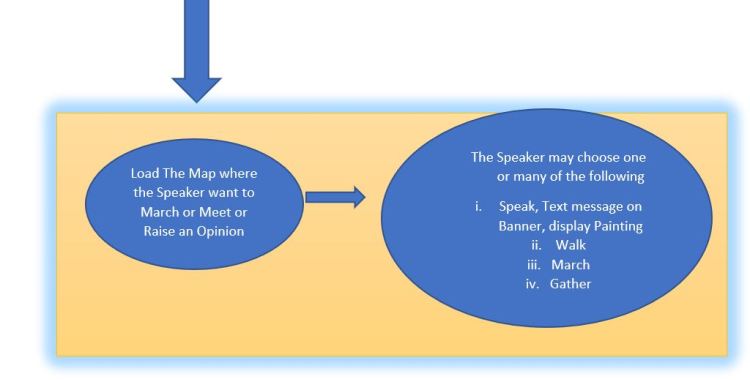
Given that typically such opinions are expressed by a group who thinks in a similar way on a particular topic. Now, this article questions and present a solution to this issue, given we have high end technologies to implement the solution. The proposed solution is based on the concept I illustrated in the beginning –game playing. Online game playing has been advanced to its peak both in technology used but also in use of Artificial Intelligence. I propose use of computer science and technology which can be implemented to enable participants from both side—speaker and hearer and from all models of one to one or one to many or many to many entities.
The entities on each side can hold the following objects
A Platform can be made where the participant can do the following.
With the advances in gaming technologies, virtual reality, augmented reality the march, celebration movement, or even a road annual party can be made virtual.
The stakeholders may take decision based on Artificial Intelligence tools and decision based on either:
a. majority votes of stakeholders
b. majority votes + user voices
c. majority votes of speakers
More on this in coming blogs.
This article presents a robust computerized – “Artificial Intelligence” based Health Care System, which works on a global level and is efficient in handling global issues such as pandemic, in a unified, co-operative international approach enabled only with help of mutual trust and understanding.
Most health care systems today are efficient and well equipped. But as the pandemic has shown us they are lacking in co-operating and efficiently dealing with the current pandemic situation from a global perspective. Here, we need a health care system with co-operates among towns & cities not just among individual care facilities and among countries not just among cities. While most health care institutions in todays world are working on stand-alone model, where networking between even two hospitals across the street is based on emails, messenger services and telephone conversations-landline or mobile. In this article I am putting a light on an approach for better inter-operability among stand-alone the systems both within towns (cities or villages) and on a global level-within countries.

Figure 1. The flowchart describes the way information can be processed and decision making using Artificial Intelligence can be applied for future medical tasks and leaderships.
It was around a decade back that global level work on Clinical Document Architecture (CDA) was proposed. We all are familiar with the term medical records which may be written by human or a computer. When the records are written on a computer it needs a format, typically called a medical description language or MDL for short. To briefly explain what CDA was all about, so that you don’t have to refer back on a search engine for that. CDA, basically in layman language, provided a standard for storing medical information of a patient. The details are stored in the format finalized by the experts, the details include, patients’ medications, disease severity, doctor specifications for medications, to diet restrictions followed and may even include the comments from the nurse in charge of the patient. There are several ways in which CDA can be written which may include PHMR (Patient Health Care Monitoring Record), CCR (Clinical Care Record) to mention a few, these are specialized forms of the model of CDA. This may be understood as different ways to input and view information based on who is accessing the data. Once the document is made at the entry of a person in hospital, it initializes the basic details counting up to height of the person, to illustrate it to you. There are xml fragments -specified by xml tags- that are updated-and/or added once a doctor has some comments or medications to prescribe to the patient. Each disease has a code—codes were added in specification for making it easy for a computer to understand the condition of a patient. Though natural languages could have been processed (and NLP could have been used), but may by then, and even now, the question of resolving ambiguity of a natural language (about a disease name, symptoms, side effects…), that too in a critical application such as health care is paramount and could not have been left to negligence of accuracy even by 0.9%. In this way the xml is updated, adding blocks of tags for each disease, symptoms, medications and so on. The initial impression of the proposed thing was the xml for a patient id may go to a centralized server, where all cumulative files about a health institution may be stored. These makes it easy for processing hospital level information. But nobody predicted a pandemic, as far as I know, so to the best of my knowledge even if these models had been implemented on some care systems, there seem to be an absence of global records and the cumulative understanding of these records.
Why global accumulations of such records can be considered necessary ? Yes, it is a question about why you are reading this article! Well, computerized documentation is being provided by many health care facilities, including individual clinics. There are names such as medical records, medical descriptions, or simple excel file based databases which are used at backend (either on a web server or a desktop application), some may be using xml files themselves. But they may lack unified approach and standards to store information. This makes it difficult to comprehend data from one server to another. Why we need to connect data from one server to another??? Well yes there was not much need for it before this – Pandemic never hit us after the Computer Revolution, as we may call it and specifically Artificial Intelligence Revolution, as I would like to call it —to what is going on now! This may be a reason why centralized approaches to store such contents were not performed. You may ask—how many of super computers can process scattered data, spread across countries, each small unit in a different form. I say—None-at present ! WHY?? Well you would need lot of human specialists efforts for writing rules for inter-compatibility of forms in which data is present –in each clinic, in each hospital, in each care house to mention a few! Basically, you need a standardized data, which no one has time to create—given such a big load on the Front Line Workers-Our health care providers! Now you may ask me – why doctors and specialists needed for this task- Well Guys—all these are medical terminology, the name of disease in a particular format, the medicine names. Check out LONIC and SNOMED codes for instance, that were recommended by some for a standardized approach. How many -medical description languages- use these standardized codes! ? Or do we need more standardized codes or are these enough ?! I think a lot of work has gone in coding medical standards, and re-usability is a popular software if not hardware jargon we all follow. The answer would be yes—if we can gather some medical coding specialist to translate the formats of MDL into a unified coding format –that can be fed into Super Computers.
The proposal was well studied and several guidelines were framed. However, it seems that not much is implemented about centralization of the medical information. Now, individual units can maintain their medical record, process it and even apply Artificial Intelligence on the data and generate analytical graphical visualizations many AI and data scientists are used to view for decision making. But here, we stand amidst, in some places on the on-set of, the third wave and second wave of pandemic. It is needed to now use medical coder—to translate the MDL files from individual units, institutions, villages, clinics and so on to a unified form as proposed years back.
The medical information may vary from
Once this information is on servers-we can do a lot of Artificial Intelligence on it and help people, not only doctors and policy makers with authentic information from reliable sources. I now propose the use of Artificial Intelligence in
Once this mission is accomplished, we have better tracking, and who knows we can track even the virus from its roots, with the help of tremendous amount of development in Artificial Intelligence that can beat humans in tough games like Chess!
More on this in my upcoming blog. Stay tuned! Take care! And Start Implementing It!
You must be logged in to post a comment.